Gridding and Contouring
Contouring requires the existence of regular grids. These grids can be pregenerated, as is the case with the GRIB files from HRS or generated by WXP from the raw data using an objective analysis scheme.
Objective Analysis
Non-gridded data must first be fit to a grid in order to be contoured. This is accomplished using a "Barnes Objective Analysis Scheme" which is done automatically within WXP's contouring programs. These programs read in and process the data, apply functions and change units prior to fitting the data to the grid. The grid is then computed using the objective analysis algorithm. Each gridpoint value is determined by calculating a weighted average of data surrounding the gridpoint. The weight for the stations can be computed as follows:
weight = exp( -r2/a )
Where:
- r -- is the radius between the data station and the gridpoint.
- a -- is the smoothing (or filter) parameter.
The filter parameter is used to determine how smooth the resulting grid will be. In general, values around 1 are used for high detail and values nearing 10 for smoother grids. Only those stations within the radius of influence (initially set to 3 grid spacings) are included in the weighted average. If no stations fall within this radius, the gridpoint value is set to missing and the resulting grid box is not contoured. Data void regions will show up as missing areas on the contour plot. The number of stations that must fall within the radius of influence for the gridpoint to be valid is defined by min_stats. This defaults to 1.
Subsequent passes through the objective analysis scheme can be performed which attempts to converge the gridpoint value to the value of the nearest station. The second pass is done by bilinearly interpolating station values from the derived grid and computing residuals. Then these station residuals are fit to the same grid and resulting values used to correct the gridpoint values. On the second pass, a convergence factor is applied to the filter parameter to speed up convergence. A drawback of a one pass Barnes scheme is often that maximum and minimum values are smoothed over. The benefit of the second pass is to reestablish the maximum and minimum points in the grid but this is often at the expense of creating a noisy gridded field. Gridding statistics along with RMS errors are displayed if the message level is set to "out3".
            ********************************
            *      grid  information       *
            ********************************
Time and date are            = WXP analysis for 04Z  3 JUN 97
Data field 1                 = Surface Temperature (F)
Number of stations           =  208 stats
Central latitude             =   43.0000 deg
Central longitude            =  -93.0000 deg
Spacing between grid points  =    1.1000 cm
Number of grid points (w-e)  =   25 pts
Number of grid points (s-n)  =   17 pts
Number of passes             =    2
Filter parameter             =    1.0000 cm**2
Radius of influence          =    3.00 grids
Minimum stations at gridpt   =    1 stats

Fitting to grid...
Pass: 1...
Computing residuals...
RMS Error for field 1: 1.226064
Pass: 2...
Computing residuals...
RMS Error for field 1: 0.312472
The filter parameter, the radius of influence and number of values can be set with the object_param resource.
-oa=filter,radinf,passes,converg,min_stats
Once the gridding is complete, subsequent functions may be applied on the grids such as convergence or advection. The grid is then set to the contouring module.
NOTE: Contours over data void regions such as oceans may be erroneous. The radius of influence is provided to help locate these regions. Other types of data such as synoptic data that contain ship and buoy data can be used in these regions to help obtain more valid contours.
Grid Doubling
It may be necessary to change the resolution of a grid from the default specified in the plot_domain resource. Rather than specifying a new domain, the grid can be doubled or tripled in resolution by using the gridx plot parameter:
-pp=gridx2
will double the resolution of the grid in each direction. It does the following:
- doubles the gridpoints in each direction
- divides the grid spacing by two
- doubles the radius of influence
Other integral factors can be used such as 3, 4 or 5.
Saving Grid Files
By default, gridding programs do not save grids to file but use them internally. In order to save gridded fields to file, you must explicitly specify the output with the out_file resource. For example:
-of=wxp[:filename]
specifies to create WXP ASCII grid files. Other keywords include "wxpb" for binary WXP grid format and "cdf" for netCDF file format. The output filename is dependent on the particular grid name tag. For example, surface data uses the sfc_grd tag and the name convention is looked up in the name convention file:
sfc_grd %G/%v_%h%m%d.grd
with the output going into the directory pointed to by the grid_path resource. Often, the grid filename will contain the name of the variable (%v), level (%l) and forecast time (%f) in order to distinguish between grids. It is recommended to include these parameters in the name convention.
If desired, the output filename can be specified with the out_file resource:
-of=sfcwx.grd
The filename is first used as a file name tag and if not found in the name convention file, used as a filename with the grid_path resource value prepended to the filename. If only the filename is listed, the output will be in WXP ASCII format. If another format is desired, specify the format separated by a comma:
-of=cdf:sfc_grd.cdf
If the output is standard output, the "std" keyword can be used:
-of=std
If this is to be piped to another program, it is recommended to set the message level to "none" so that only the raw data displays. In most of these cases, the program is generating data for another program and thus does not need to plot the data. In these cases, it is recommended to turn off plotting with "-pl=none".
Contouring
To visualize the grids, a simple contouring algorithm is used. There are the following plot types:
There are several plot types available to handle these types of data.
| Plot Type | Description |
| cont | Unknown contour type. Prompt the user for the contour type. |
| cf | Use color fill contours |
| lcf | Use a combination of color fill and line contours |
| ln | Use line contour |
| dln | Use dash line contours |
| ndln | Use dashed line contours on negative values, line contours elsewhere. The con_base resource can be used to set the breakpoint. |
| gvalue | Plot the gridpoint values |
The contouring is broken down into 3 segments.
- contours -- the actual contours
- contour labels -- the labels for each of the contour lines
- local maxima/minima -- the extreme values plotted with a H and L with appropriate values
Color Fill Contours
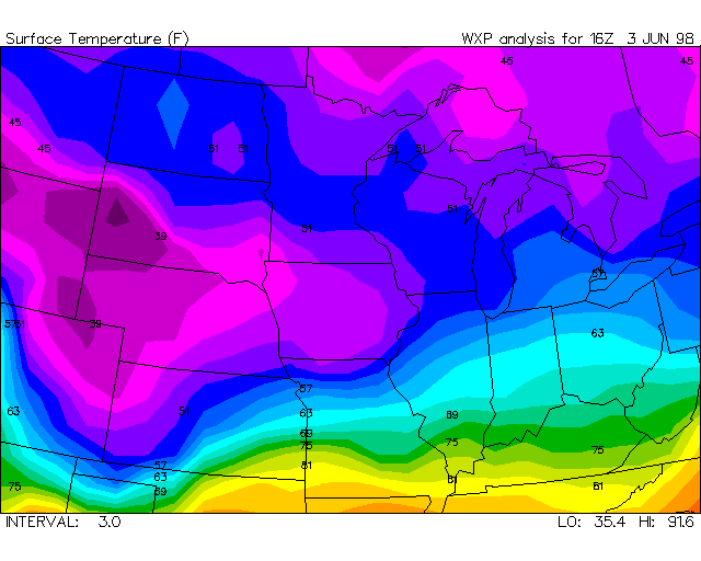
A color fill contour plot will fill areas between contour lines with a specific color. By default, these 15 colors are:
magenta, lmagenta, blue, lblue, cyan, lcyan, green, lgreen, brown, yellow, red, lred, dgray, lgray, white
The lowest contour value will be filled with magenta and the next highest with light magenta and so on. If there are more than 15 contour levels, the colors will wrap around to magenta again. If necessary, the user may select the color fill colors with the color_fill resource (up to 256 colors can be listed). To obtain the best color fill plot, the user should take care in selecting a contour interval so that around 15 contour levels are displayed. In other words, take the difference between the maximum and minimum, divide by 15 and round up (see automatic intervals).
To not plot a contour level, use "off" for the color. This is useful in overlays. Also, fill patterns can be used to make the contours translucent. A sample plot:
   sfccalc -cu=la -re=mw -va=temp -in=3
-pl=cf -de=d

Since the first color fill color is linked to the lowest value in the grid, looping these images may result in color variations from plot to plot. Using the con_base resource locks in the colors at a specific value so that loops will have consistent colors.
Line Contours
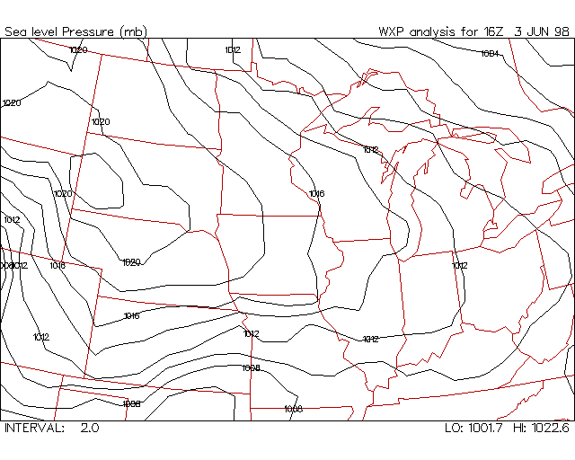
There are several types of line contour plots. There are straight line contours (ln), dashed line contours (dln), negative dashed line contours (ndln) and color fill and line contours (lcf). When a negative dash line contour type is used, the break-off point between line contours and the dashed contours is 0. Line contours exist at this value and above. Dashed contours appear below this value. The con_base resource is used to set the break point if it is not 0. A sample is:
   sfccalc -cu=la -re=mw -va=pres -in=2 -pl=ln
-de=d

By default, all line contours are drawn with the same color and the same attributes. By specifying the color_fill resource, the attributes in the color fill resource will carry over to the line contours. The first attribute is linked to the lowest contour. If the color_cont is set to "off", the colors from the color_fill resource will be used as well.
Smooth Contours
The WXP contouring algorithm does not smooth contour lines after computing them. Adding spline interpolation sometimes does not give reasonable contours. To get smoother contours, double the gridpoints in the domain. To double the gridpoints, use the "gridx" plot parameter (see grid doubling above). Keep in mind that object analysis parameters ought to be changed as well. The radius of influence should be doubled along with a small increase in the filter parameter:
-pp=gridx2 -oa=2,6
Tripling the gridpoints can give even better results but can produce plateau effects. Make sure the number of stations going into the objective analysis is enough to merit the increase in resolution by increasing the station priority.
Gridpoint Values
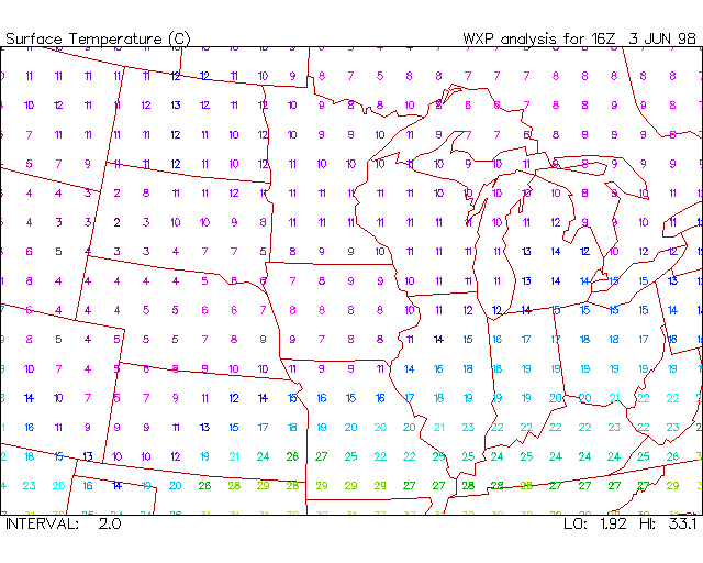
If the "gvalue" plot type is specified, the output will be plotted values at each gridpoint. The color of the plotted data is controlled by the color_cont resource. If a contour interval is specified, the values are colored based on their values. The contour base can also be set to lock the colors to a specific value range. To format the values, the plot_format resource can be specified. A sample plot:
   sfccalc -cu=la -re=mw
-va="temp[C:gvalue:in=1]" -de=d

Contour Line Labeling
The contouring routine automatically labels every other contour line only when the contour passes through opposite sides of a grid box. The labels are limited by a skip factor in X and Y. By default, these line labels appear once every nx/5 grid boxes in X and ny/5 grid boxes in Y. For a 25x17 grid, this is every 5 grid boxes in X and 3 in Y. This limits the number of contour labels that get drawn.
Local extremes are also plotted. By default, the extremes are labeled whenever a gridpoint is the minimum value of all the gridpoints that are within 2 gridpoints of that gridpoint for a total of 25 gridpoints. If the value is the maximum value within those 25, it gets an "H" label with the appropriate gridpoint value. If it is the minimum value, a "L" is plotted along with the value.
The labels specification can be adjusted with the lab plot param. The syntax is:
lab=Lab[:Rad][:X][:Y]
where Lab is the number of contour lines between labels. The labels start at the lowest value or the value of con_base and, every Lab'th line is labeled. The default is every other line. Rad is the search radius for local extrema. The default is 2 gridpoints in each direction. The X and Y values specify how many gridpoints in X and Y to skip between labels on a specific contour line where the default is nx/5 and ny/5.
Line labels can be turned off if Lab is 0. If this is the only value specified, both labels and extrema are turned off. If Rad is 0, the extrema are not plotted.
The colors and attributes for the labels are defined by the color_label resource for line contours and color_clabel resource for color fill contours. By default, the line labels are in white and the fill labels are in black.
Overlay Map
The map is then overlaid in black. The map color and attributes can be changed with the color_map resource for line contours and the color_cmap resource for color fill contours. The defaults are red for line contours and black for color fill contours.
Color Bar
A color bar can be displayed on the image if the "bar" plot parameter is set. It automatically appears if irregular contour values are specified with the color_fill resource. The bar is drawn in the lower left corner of the plot and shows the colors used in the color fill plot labeled with their associated values:
![]()
Plot Attributes
Plotting attributes affect how the data will be contoured. The types of attributes available include color and fill pattern.
Resources
The color, line width, text size and scale factor can be set with the following resources:
- color_cont - for line contours
- color_fill - for fill contours
- color_label - for line contour labels
- color_clabel - for fill contour labels
- plot_format - for specific formatting
- con_interval - for coloring plotted data
- con_base - for setting range and base color value
- plot_param - for extra plotting parameters
Variable Specification
Other attributes can be changed when specifying the variable or in the variable file. When specifying a variable, the following syntax is used:
[time:level]varname[[units[:attributes...]]]
The time and level parameters are the same as can be specified with the time and level resources. These are often specified with these resources and therefore are optional. The units and attributes are surrounded with brackets "[ ]".
Units
The input data will have a specific set of units that can be modified by specifying the units within the brackets. For example, to change the temperature to Celsius:
-va=temp[C]
The list of available unit conversions is in the units.lup file (See the units conversion section of the Users Guide).
Attributes
The attributes are listed after the units. Multiple attributes can be specified separated by colons ":". For example, to plot temperature in C, using blue line contours:
-va=temp[C:ln:co=blue]
Here is a list of available attributes to specify:
| Attribute | Description |
| type | The type of plot: cf, lcf, ln, dln, ndln, gvalue |
| %format | Specifies the printed format of the data. This is a full C format such as "%7.2f". The default is "%.0f" or zero decimal places. |
| mx=max | Specifies the maximum value in the contour plot. All values greater than this value will not be plotted. |
| mn=min | Specifies the minimum value in the contour plot. All values less than this value will not be plotted. |
| co=color | Specifies the color. This is the color name from the color table. If this is the first attribute, the "co=" may be omitted. |
| wi=width | Specifies the width of lines. This includes lines used in text and markers. The default value is 1.0. |
| st=style | Specifies the style of lines. Possible values are:
|
| fo=font | Specifies the font number. See the font_list resource. |
| fi=fill fp=fill |
Specifies the fill pattern. Possible values are:
|
| sc=scale | Specifies the scale factor. Most drawn data is scaled by this parameter. The default value is 1.0. |
| hi=height | This is the height of text and the size of markers. The default value is 1.0. |
| te=expan | Specifies the text expansion factor. This controls how wide text is plotted. An expansion factor greater than 1 results in fat text. A value less than 1 results in thin text. The default value is 1.0. |
| in=intrvl | Specifies the contour interval. |
| cb=base | Specifies the contour base value. The default is the minimum value of the grid. |
| cof=file | Specifies a color fill attribute file to use for color fill parameters. |
| lab=lab.rad.X.Y | Specifies the contour labeling options. See the contour label section above. |
| labs | Specifies to use simple labels (level varabbr (unit)) |
| bar | Specifies to display a color bar. |
Automatic Intervals
By specifying zero (0) as the contour interval, a reasonable interval is computed based on the number of values in the color fills (see color_fill resource).
interval ~= (max-min)/num_colors
This value is rounded up to the nearest whole number. This is also based on the range of data so if the range is less than 1, the program will make the resulting contour interval a fractional value.
Maximum Number of Lines
In some cases, the contour interval is specified so small that hundreds of contour lines will be drawn on a plot. This can also occur if there is bad data, which is commonly referred to as a bulls-eye. This can cause problems for the contouring algorithm if it has to draw all these lines. As a result, there is a limit to the number of lines that can be drawn within on grid box. The default number is twice the number of color fill colors. If this is not desirable, the maximum can be reset with the "maxl" plot parameter:
-pp=maxl:75
If the factor is less than 0, it is a multiplier of the number of color fill colors. For example (using 20 color fill colors):
-pp=maxl:-5
would yield at most 125 lines in a grid box.
Last updated June 1, 1998