Upper Air Data Analysis

Upper Air Plotting

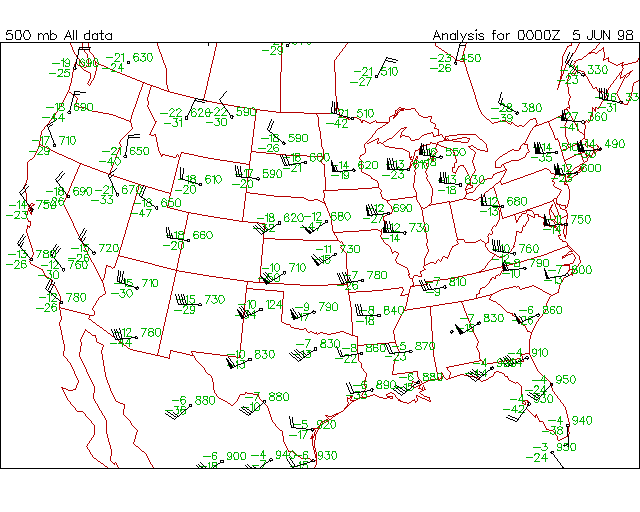
Upper air data may be plotted with the upairwx program. This program works much like the surface plotting program, except upper air data are sparse and relatively evenly spaced, so that subregional displays and station prioritization are not needed. Instead, a specific pressure, height or isentropic level must be picked.  In general, pressure levels are picked ranging from the surface to 10 mb including tropopause and maximum wind levels. If the level is not a mandatory level, the data will be interpolated from a merged sounding including mandatory and significant level data. Once the level has been selected, the menu listing the available upper air variables to be plotted is displayed. These variables represent raw data stored in the upper air converted files plus several derived variables. Some variables like temperature can be averaged over a layer "850-500mb" where the layer is specified as the level.  Others are only valid at specific levels such as station pressure and 1000-500 mb thickness.  These variables are available on the sounding level.  A composite upper air station plotting model is:

and a sample composite plot is:

upairwx -cu -le=500 -va=all -de=d 

Upper Air Gridding and Contouring

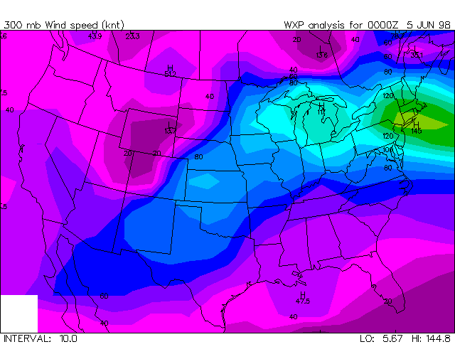
The upper air gridding and contouring program is upcalc. This program works in the same manner as the surface gridding program and the upper air data plotting program. A pressure level is selected for gridding and the variables represent the input data plus derived variables such as potential temperature, vapor pressure, mixing ratio and relative humidity. Once a level and variable have been selected, the gridding and contouring are performed. Wind vectors and streamlines of upper air data may also be plotted.

upcalc -cu -le=300 -va=wspd -pl=cf -in=10 -ct=rainbow.clr -cof=0-23 -de=d 

Upper Air Sounding Calculations and Plotting

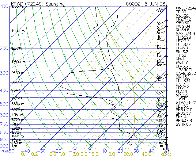
Vertical sounding information for a particular station can be displayed by using the uacalplt program. This program reads in data for a specific upper air station, lists the data, performs standard sounding calculations and plots the sounding on one of the following:

• Skew-T log-P -- an energy conserving diagram in which the temperature and potential temperature lines are perpendicular. In this diagram, the temperature lines are offset at a 45 deg angle sloping to the upper right.  And example of a skewt is below.
• Emagram -- an energy conserving diagram similar to the Skew T except that the temperature lines are not skewed to the right.
• Stuve -- not an energy conserving diagram but one where potential temperature lines (adiabats) are straight.
• Hodograph -- displays winds with height on a polar grid. On this plot, the wind direction is the angle and the wind speed is the radius from the center. Concentric circles are plotted at 20 knot intervals for easier definition of actual wind speed. Also, the plot is annotated with the mandatory level pressure above and to the right of the location of the wind.

Each different type of line is represented by a different color. The horizontal blue lines represent pressure lines while the vertical blue lines are temperature lines. The sloping green lines are dry adiabats or the lines air parcels follow when lifted. The sloping cyan lines are moist adiabats which represent the lines air parcels follow when saturated and releasing latent heat. The dashed yellow lines are mixing ratio lines which represent moisture content in the atmosphere. The sounding data are displayed in white with the left white line representing the dewpoint line and the right line representing the temperature line. The wind barbs on the right edge of the diagram represent the winds at various elevations with the top of the diagram representing compass north. The winds at mandatory levels are plotted at their pressure levels, whereas the winds at height levels are plotted at their standard atmosphere pressure level. Also, a parcel trajectory drawn as a yellow line is added to the thermodynamic plot to reflect sounding stability.

uacalplt -cu -id=KFWD -me=out2 -pl=skewt